


Look for a common driver before linking ocean series
Strong correlation and a plausible lead can arise when two ocean records share a driver rather than directly influence one another. This methods note combines Earth-system causal-inference research with studies of nonlinear ecological dynamics and autocorrelated fish-environment data. An invented two-regime calculation produces a correlation of approximately 0.94 despite zero within-regime association and no constructed direct effect. The analysis then examines lagged common forcing, sampling and smoothing, seasonal transformations, adjustment choices, and the assumptions behind advanced causal methods. It attributes no actual ocean event and does not claim that conditioning alone establishes causation. Its practical outcome is a sequence of rival physical explanations and discriminating observations, allowing unresolved associations to guide a better next measurement instead of an overstated causal story.
Sea-ice forecast skill starts with a baseline
Forecast accuracy does not establish added information unless it is compared with an explicit alternative. This methods note draws on primary ice-edge verification and subseasonal prediction studies to define a fair comparison among a model, climatology, and persistence-based forecasts. A hypothetical Brier-score calculation shows how a model can be skilful against one baseline and unskilful against another. A spatial example explains why correct total extent can coexist with a misplaced ice edge. The note examines issue-time information boundaries, changing climatology, calibration, dependence, and observation uncertainty without evaluating an operational system. Its practical conclusion is a conditional skill statement naming the target, lead, dates, region, reference observations, and baseline, rather than treating a high percentage of correct outcomes as sufficient evidence of usefulness.
What a decibel number needs beside it
A decibel value becomes comparable only when its physical quantity, reference, frequency support, averaging interval, and calibration are known. This methods note synthesises laboratory guidance and acoustic-methods research to distinguish sound pressure level, peak measures, sound exposure, and spectral density. Hypothetical calculations explain the conventional reference difference between air and water, the effect of duration on exposure, and why averaging logarithmic levels can differ from an energy-equivalent average. The discussion also separates received levels from source levels and pressure measurements from particle motion. It does not establish current regulatory thresholds or biological equivalence between equal exposures. The practical result is a reporting minimum that prevents an apparently precise acoustic comparison from concealing different quantities, processing choices, or measurement limits.
When conductivity does not mean saltier water
A conductivity change is not a direct measurement of changing salt content because temperature, pressure, units, and seawater composition affect its interpretation. This methods note follows the documented TEOS-10 calculation chain from conductivity to Practical Salinity and Absolute Salinity, then to thermodynamic interpretation. A published Gibbs SeaWater demonstration supplies two nearly equal conductivities with substantially different calculated salinities, making the importance of context explicit. Hypothetical archive and mooring cases show how a convention change can create an artificial step and why validated freshening does not uniquely identify its source. No field deployment or calibration is analysed. The note identifies the variable definitions, original inputs, processing versions, and quality information needed before a profile can support claims about water masses, density, or freshwater pathways.
From ocean heat flux to a conditional melt bound
Converting an ocean heat flux into centimetres of ice can check physical scale without predicting sea-ice loss. This methods note uses published ocean-ice heat-budget research and the TEOS-10 framework to derive a conditional latent-melt equivalent. A hypothetical flux of ten watts per square metre over thirty days supports approximately 8.6 centimetres under explicitly simplified property and energy-allocation assumptions. Further cases show how conductive export, duration, area denominator, and reduced winter growth change the interpretation. The note distinguishes a bound on one specified energy contribution from an unconditional bound on total melt. It does not estimate a present Arctic flux or attribute observed retreat. Its reporting framework keeps system boundaries, counterfactuals, thermodynamic approximations, and unmeasured transport beside the calculation.
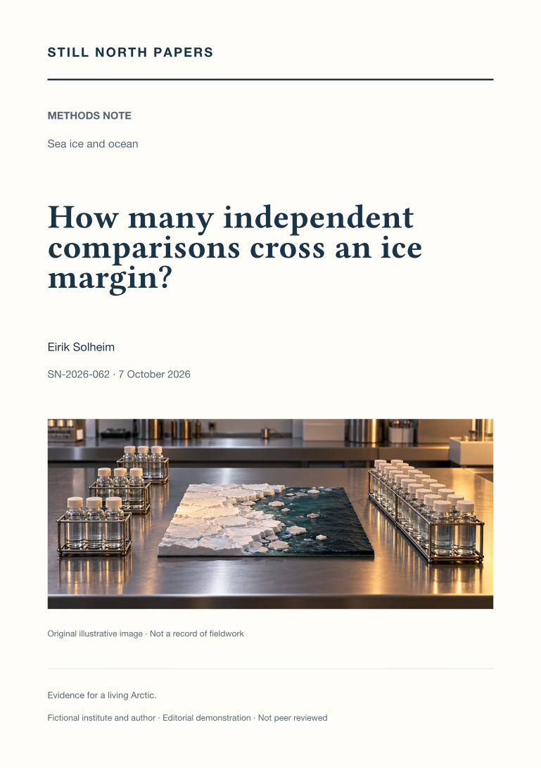
How many independent comparisons cross an ice margin?
An ice-margin transect can contain many samples but only one independent environmental contrast. This methods note combines published principles of replication with Arctic bloom observations to examine how a limited station budget can support a defensible regional question. A hypothetical allocation of eighteen casts compares a dense single crossing with three repeated crossings, distinguishing technical replication, local gradient resolution, and variation among contrasts. The note also separates distance from the present ice edge from time since local retreat and examines sampling order, depth integration, water masses, and access-related missingness. It offers neither a cruise plan nor a power calculation. The useful conclusion is an explicitly bounded association whose claimed replication matches the field design rather than the number of bottles collected.
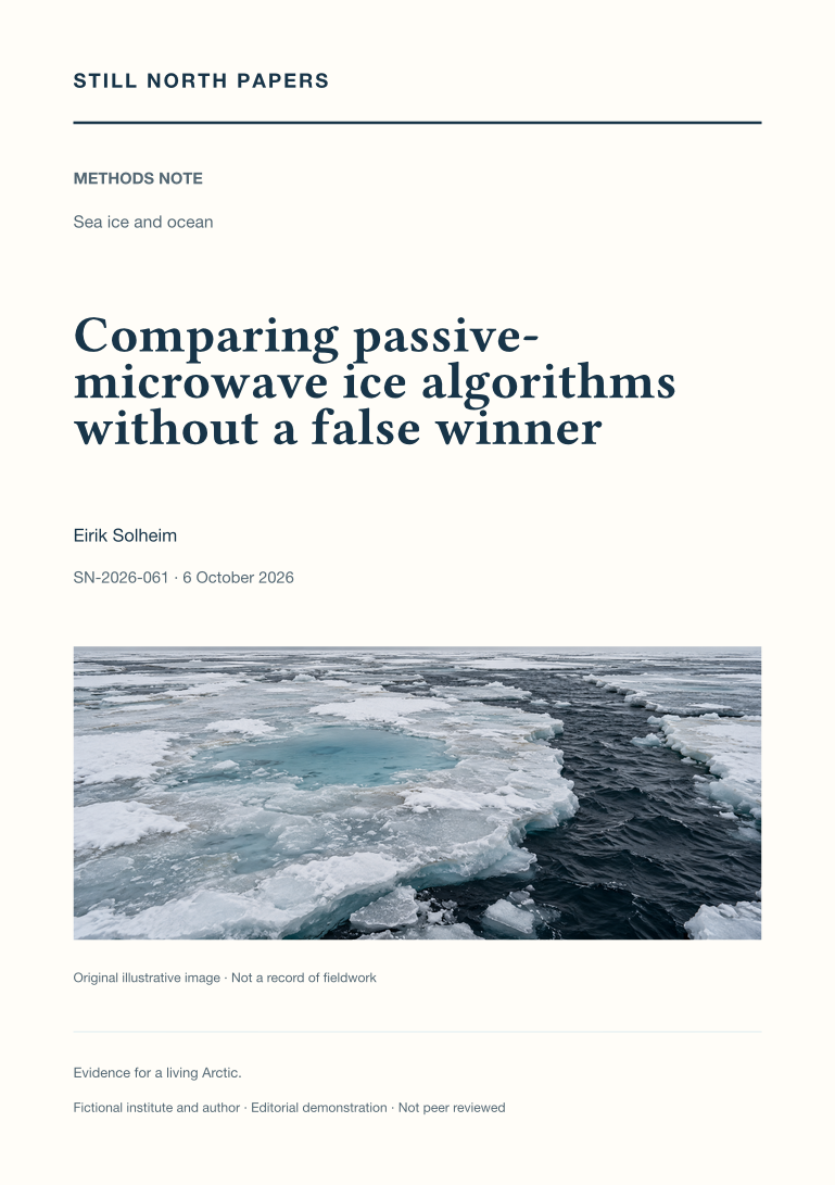
Comparing passive-microwave ice algorithms without a false winner
Passive-microwave sea-ice products can disagree because their retrievals, calibration, filtering, and surface assumptions differ. This methods note synthesises three published intercomparisons to show how a fair quantitative evaluation separates bias, scatter, spatial cancellation, and threshold effects. Invented matched-footprint examples demonstrate why zero average error can coexist with local errors, why clipping at full concentration can conceal retrieval bias, and why a small concentration difference can produce a large extent difference. The analysis distinguishes concentration from net ice surface fraction and treats summer melt as a separate evaluation problem. It does not rank current operational releases or rerun the cited studies. Its practical outcome is a conditional product comparison tied to a stated quantity, season, reference dataset, and downstream decision.
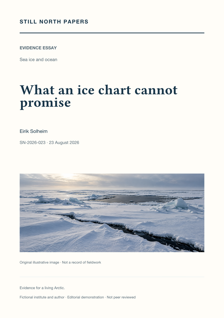
What an ice chart cannot promise
Regional ice charts are read as time-referenced analyses, not guarantees of connectivity, strength, or safe travel. The essay uses Canadian Ice Service documentation to distinguish observation, publication, and valid times, and to explain concentration, stage-of-development, and floe-form information in the egg code. An invented mixture demonstrates why partial concentrations describe an area rather than a sequence along a route. Drift, deformation, unresolved fractures, and separate iceberg information expose the limits of promoting one chart into a complete hazard map. Climate anomalies are also distinguished from operational permissions. No route or thickness recommendation is offered. The useful outcome is a complete product retained with its legend, source, time, and coverage, alongside recognition of the local competence, authority, and current information a journey would additionally require.
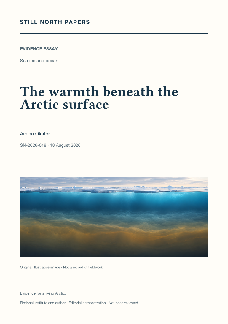
The warmth beneath the Arctic surface
Subsurface Arctic warmth is examined through the density structure that separates a heat reservoir from the ice above it. The essay explains how salinity can keep warmer Atlantic-origin water beneath a colder, fresher surface layer and uses contrasting hypothetical columns to distinguish stored energy from access to that energy. Heat content, horizontal transport, and upward flux are treated as separate quantities requiring different observations. Published Atlantification evidence supplies regional contrasts rather than a claim that the entire Arctic has lost its stratification. The discussion connects upward heat transfer with reduced winter ice growth and potentially changed nutrient supply, without prescribing one ecological outcome. Temperature, salinity, velocity, mixing, depth, and position are therefore needed to follow the mechanism from incoming water to a measured effect at the surface.
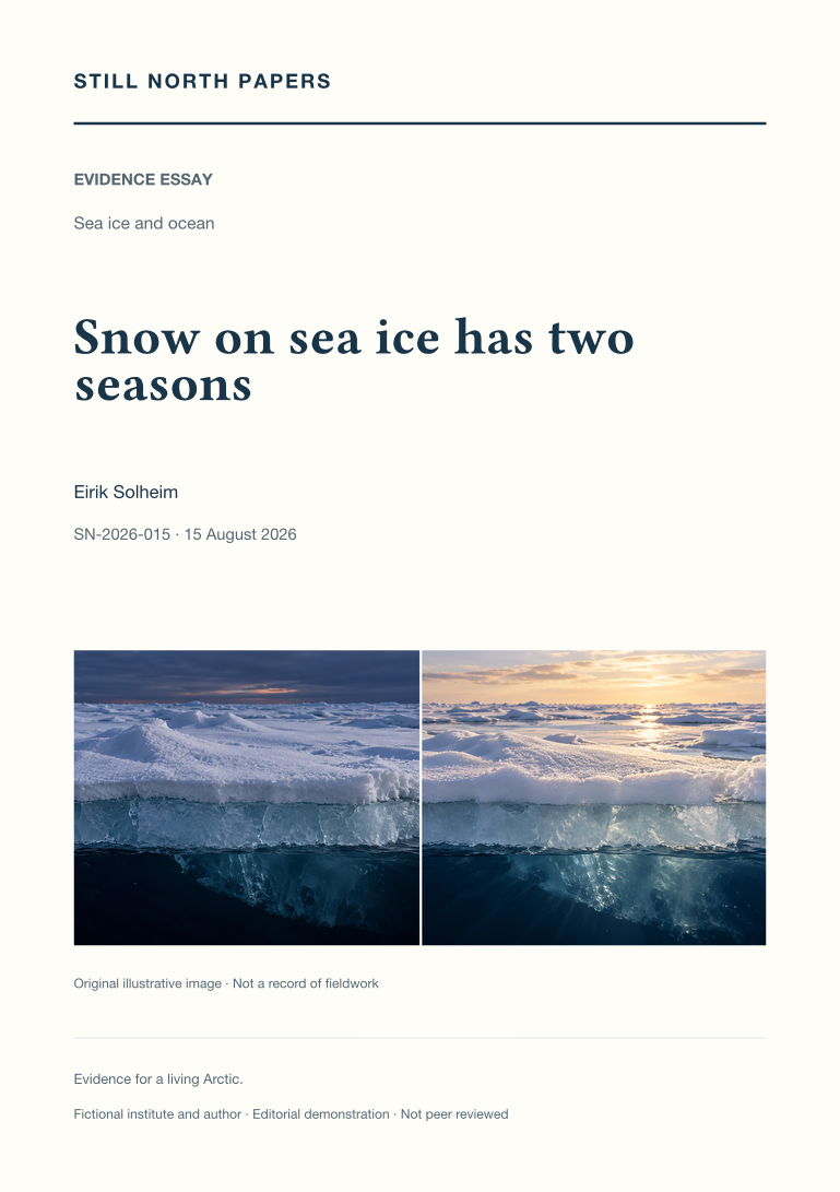
Snow on sea ice has two seasons
Snow on sea ice changes two seasonal energy pathways: it can restrict winter heat loss and ice growth, then reflect sunlight and delay spring melt. A controlled hypothetical comparison isolates the insulating effect without pretending to predict the fate of real floes. The essay shows why snowfall timing, depth, density, grain structure, and wind redistribution matter, and why melt onset is not equivalent to ice disappearance. It also examines the role of snow assumptions when satellite elevation is converted into ice thickness. Neither a convenient drift measurement nor a single seasonal slogan can determine the annual net effect. Useful observations connect surface type, date, weather, ice thickness, and a documented sampling route, allowing apparently opposing findings to be read as parts of one seasonal account.
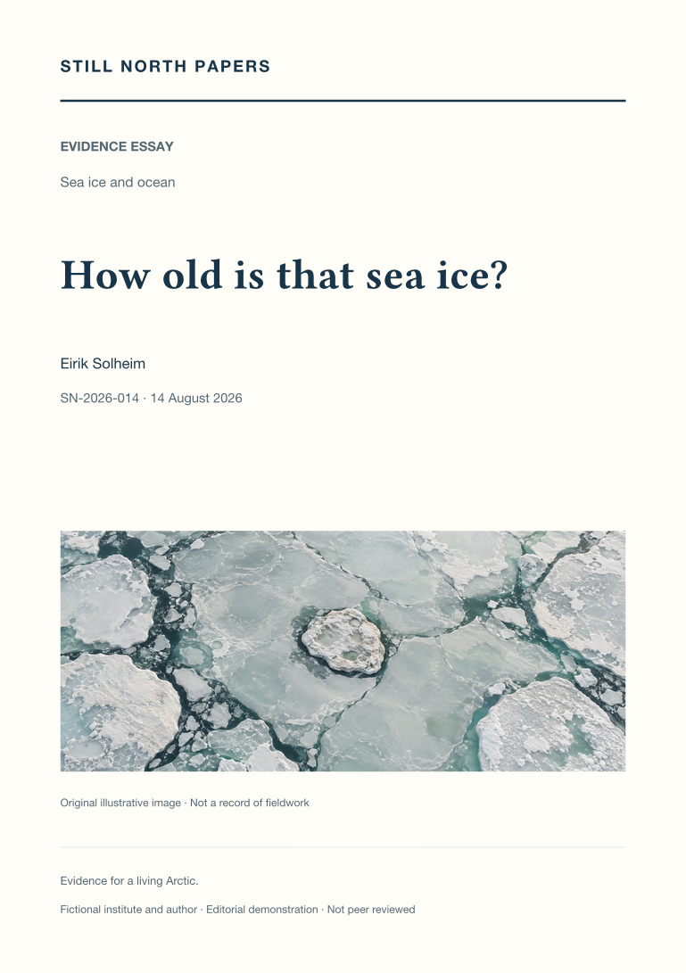
How old is that sea ice?
Sea-ice age is interpreted as a reconstructed history of survival and movement rather than a direct map of thickness or strength. The essay explains first-year and multiyear categories, parcel tracking, and the important product rule that retains only the oldest category within each grid cell. A hypothetical mixture demonstrates why identical colours need not imply identical fractions of older ice. Deformation, melt, snow, and travel history further limit age as a thickness proxy. The published decline in the oldest category is retained with its late-summer timing and comparison period, while the need for successive summer survival explains why a winter extent rebound cannot immediately rebuild old ice. The resulting reading method asks for product, week, categories, and compatible complementary measurements, not a promise about travel or habitat.

Extent and volume tell different ice stories
Extent, area, and volume are separated through a hypothetical sea-ice grid cell whose concentration and thickness can change independently. The worked arithmetic shows why an unchanged outline can conceal a loss of frozen material, while wind-driven spreading or compaction can alter extent without equivalent ice formation or melt. The essay explains the concentration threshold behind extent, surface-melt complications in remote sensing, and the sampling problem posed by thickness distributions. PIOMAS is described as a model-based reanalysis with validation and uncertainty, not a direct weighing of the pack. Published seasonal extent results provide an example of how rankings can be overextended. A fair comparison retains dates, domains, units, reference periods, and the meaning of uncertainty before deciding whether apparently conflicting graphs are physically consistent.
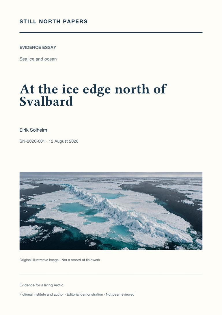
At the ice edge north of Svalbard
Using an explicitly illustrative scene north of Svalbard, this essay examines how an ice-edge observation becomes evidence without becoming a claim about the whole Arctic. Pressure ridges expose the sampling problem of unusually thick features, while melt ponds show why date, drainage, weather, and surface geometry matter to comparisons. The published sea-ice record supplies regional context for a younger ice cover, rather than results attributed to fictional fieldwork. Distant polar-bear and kittiwake observations introduce wildlife protocols, observation effort, and the limits of inferring habitat or breeding outcomes from brief encounters. The account concludes that representative sampling, matched scales, safe stopping decisions, and a documented handover are more informative than an apparently complete photographic story.